At 3 am on Sunday, 1 August 1982, a group of Kenya Air Force soldiers led by Senior Private Hezekiah Ochuka attempted to overthrow President Daniel arap Moi’s government. The Kenyan Army foiled the attempt, and President Moi’s government remained in power, although about 100 soldiers and more than 200 civilians died that day. This event would significantly influence the future of Kenya.
Instability in a country involves political, social, or economic upheaval. It manifests as a coup or other illegal regime change, breakdown of institutions, widespread systemic corruption and state capture, organised crime, loss of territorial control, economic crisis, large-scale public unrest, and involuntary mass population displacement, including war, civil war, or other forms of conflict.
I am fascinated by how society behaves, evolves, and reacts to external and internal events, as well as machine learning. Therefore, I decided to develop a machine learning model that can predict coups based on historical and socio-economic data.
Factors that lead to economic instability
- Full democracies are least likely to undergo significant political upheaval and instability. Countries undergoing political transitions face high risks of political instability and violent conflict. Luckily, the Economist Group publishes an annual democracy index that tracks the quality of democracy per country. The lower the value, the worse the democratic standards. Denmark, for example, had a near-perfect 9.28 (full democracy) while Syria had a dismal 1.32 (authoritarian) in 2024.
- Democracy is often preceded by economic development, but this alone is not enough to sustain a democracy, especially in the presence of natural resources like oil, which lends massive financial resources to the regime. A study conducted in the period 1950-1990 showed that no democracy with a per capita income above US $6,000 (in 1985 prices) has had its democratic system collapse. However, economic growth neither leads necessarily to democratisation nor to improvements in other aspects of governance. For our investigation, this means that we will have to find data on GDP per capita to measure the economic development of countries.
- As hinted at before, immense natural resource wealth like oil deposits can retard democratisation, by increasing the resources available to authoritarian regimes and simultaneously reducing the need for ruling elites to be responsive to the needs of their citizens. For this, we found a dataset of all oil-producing nations to represent natural wealth deposits.
- The history of a coup is also a factor that will contribute to a future coup. Violence begets violence, and conflict breeds more conflict. This is our main focus, and we got data from Kaggle.
- High inequality also fuels tensions and conflict. Here we will use the Gini Index as published here. This index measures the income distribution of a country, i.e. the gap between the rich and the poor. The lower the score, the more equal the country and vice versa.
Datasets
- Historic Data(previous coups) : Kaggle
- Economic/GDP Data: World Bank
- Democracy Index : Economist Intelligence and Wikipedia
- Oil Deposits in Countries : Wikipedia
- Inequality Data (class & tribal): gini index
- List of all the countries in the world: Wikipedia
Importing the Libraries and Loading the Dataset
import pandas as pd
import numpy as np
import matplotlib.pyplot as plt
import matplotlib
# from numpy import isnan

from sklearn.tree import DecisionTreeClassifier
from sklearn.model_selection import train_test_split
from sklearn import metrics
from sklearn.metrics import accuracy_score

import seaborn as sns
sns.set_style("whitegrid", {'axes.grid':False})

import warnings
warnings.filterwarnings('ignore')
%matplotlib inline

# load the goggle drive connector
from google.colab import drive
drive.mount('/content/drive')

# read the data
df = pd.read_csv(r'/content/drive/MyDrive/Coup_Data_v2.0.0.csv')
df.sample(10)
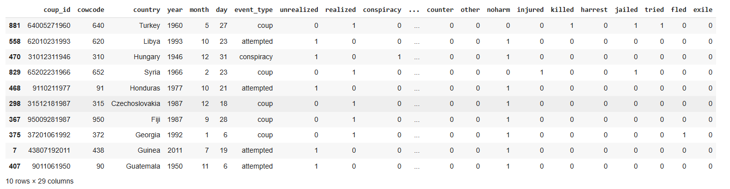
Exploring the Data (EDA)
The column ‘realized’ when equal to 1, and ‘coup’ mean the same thing.
df.columns
Index([‘coup_id’, ‘cowcode’, ‘country’, ‘year’, ‘month’, ‘day’, ‘event_type’, ‘unrealized’, ‘realized’, ‘conspiracy’, ‘attempt’, ‘military’, ‘dissident’, ‘rebel’, ‘palace’, ‘foreign’, ‘auto’, ‘resign’, ‘popular’, ‘counter’, ‘other’, ‘noharm’, ‘injured’, ‘killed’, ‘harrest’, ‘jailed’, ‘tried’, ‘fled’, ‘exile’], dtype=’object’)
df.shape
(943, 29)
There are 943 events recorded in the dataset.
df.info()
<class 'pandas.core.frame.DataFrame'>
RangeIndex: 943 entries, 0 to 942
Data columns (total 29 columns):
# Column Non-Null Count Dtype
--- ------ -------------- -----
0 coup_id 943 non-null object
1 cowcode 943 non-null int64
2 country 943 non-null object
3 year 943 non-null int64
4 month 943 non-null int64
5 day 943 non-null int64
6 event_type 943 non-null object
7 unrealized 943 non-null int64
8 realized 943 non-null int64
9 conspiracy 943 non-null int64
10 attempt 943 non-null int64
11 military 943 non-null int64
12 dissident 943 non-null int64
13 rebel 943 non-null int64
14 palace 943 non-null int64
15 foreign 943 non-null int64
16 auto 943 non-null int64
17 resign 943 non-null int64
18 popular 943 non-null int64
19 counter 943 non-null int64
20 other 943 non-null int64
21 noharm 943 non-null int64
22 injured 943 non-null int64
23 killed 943 non-null int64
24 harrest 943 non-null int64
25 jailed 943 non-null int64
26 tried 943 non-null int64
27 fled 943 non-null int64
28 exile 943 non-null int64
dtypes: int64(26), object(3)
memory usage: 213.8+ KB
This dataset had data on instability events, including coups, conspiracies, etc. We shall focus only on coups as they are an obvious measurable event and they are the worst form of regime change.
pd.pivot_table(df.sample(10), values = 'realized', index=['country'])
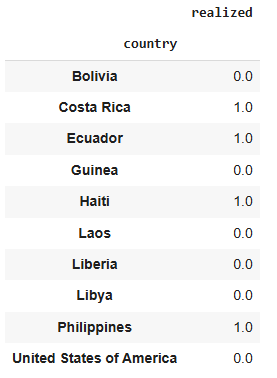
The column ‘realized’ when equal to 1, and ‘coup’ means the same thing. We shall now slice the dataframe to include only coup events, then we shall count the coups per country.
final_coups = coups.iloc[2:,2:6]
final_coups.head(10)

We don’t need the dates.
final_coups.drop(['year','month','day'], axis='columns', inplace=True)
# then we can group by 'country'
final_coups.groupby(['country'])['country'].count()
| country | |
|---|---|
| Afghanistan | 8 |
| Algeria | 7 |
| Angola | 1 |
| Argentina | 9 |
| Azerbaijan | 2 |
| … | … |
| Venezuela | 4 |
| Yemen | 1 |
| Yemen Arab Republic | 3 |
| Yemen PDR | 4 |
| Zimbabwe | 1 |
To clean this up, we need to drop the added index, then reset it and insert proper column names.
# remove index name
country_coups.index.name = None
# reset the index
country_coups = country_coups.reset_index()
# insert the column names
country_coups.columns = ["country", "Number_of_coups"]
| index | country | Number_of_coups |
|---|---|---|
| 69 | Paraguay | 6 |
| 44 | Honduras | 7 |
| 8 | Brazil | 5 |
| 90 | Thailand | 11 |
| 73 | Portugal | 3 |
| 31 | Ethiopia | 7 |
| 51 | Laos | 7 |
| 4 | Azerbaijan | 2 |
| 3 | Argentina | 9 |
| 87 | Swaziland | 1 |
| 92 | Tunisia | 3 |
| 88 | Syria | 13 |
| 15 | Chile | 1 |
| 20 | Costa Rica | 2 |
| 80 | Sao Tome and Principe | 2 |
| 21 | Cote d’Ivoire | 2 |
| 64 | Niger | 4 |
| 102 | Zimbabwe | 1 |
| 94 | USSR | 2 |
| 63 | Nicaragua | 2 |
This looks much better. Let’s make sure we don’t have any missing values.
country_coups.isna()
| index | country | Number_of_coups |
|---|---|---|
| 0 | false | false |
| 1 | false | false |
| 2 | false | false |
| 3 | false | false |
| 4 | false | false |
| 5 | false | false |
| 100 | false | false |
| 101 | false | false |
| 102 | false | false |
No missing values.
#Checking for duplicate values
country_coups.duplicated().sum()
np.int64(0)
Good, no missing values or duplicates.
Next, we get a list of oil-producing countries. I have an R script that is short and sweet for scraping Wikipedia data.
# load the rvest library
library(rvest)
oilurl = read_html('https://en.wikipedia.org/
wiki/List_of_countries_by_proven_oil_reserves')

# extract a list of tables in this page
oil_tables = html_table(oilurl)
oil_tables

# select the right table
oil_countries = data.frame(oil_tables[2])
oil_countries
getwd()

# save the table locally as a csv file
setwd('C:/Users/me/coup')
write.csv(oil_countries, 'oil_countries.csv', row.names = TRUE)
dim(oil_countries)
This yields a table that looks like this:
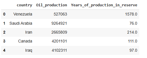
We do not need the production capacities, just a list of oil-producing nations. We will drop all the extra columns and create a column ‘oil_producing’ which we will fill with 1 for an oil-producing nation and 0 for the others.
oil_countries.drop(['Oil_production',
'Years_of_production_in_reserve'], axis = 1, inplace=True)
oil_countries['oil_producing'] = 1
oil_countries.to_csv('/content/drive/MyDrive/oil_countries.csv')
oil_countries.sample(5)
| index | country | oil_producing |
|---|---|---|
| 34 | Australia | 1 |
| 20 | Azerbaijan | 1 |
| 90 | Belize | 1 |
| 24 | India | 1 |
| 75 | Japan | 1 |
On to the Gini Index. To get the data, I did the same thing as the oil-producing countries’ data and loaded it into my notebook. This data also came with population data, which I will leave in there.
# Data on inequality as measured by the gini index
gini_index = pd.read_csv(r'/content/drive/MyDrive/gini.csv')
gini_index.head()
| index | population | country | gini_index |
|---|---|---|---|
| 11 | 52085168 | Colombia | 51.3 |
| 71 | 1425671352 | China | 38.5 |
| 75 | 334506 | Vanuatu | 37.6 |
| 94 | 654768 | Luxembourg | 35.4 |
| 117 | 3210847 | Bosnia and Herzegovina | 33.0 |
Next was the democratic index data and I got it the same way as the others. Here is a sample.
| index | country | democracy_index |
|---|---|---|
| 0 | Afghanistan | 0.32 |
| 1 | Albania | 6.41 |
| 2 | Algeria | 3.66 |
| 3 | Angola | 3.96 |
| 4 | Argentina | 6.85 |
Finally, I got a list of all countries in the world to compare against. Looking at all these disparate datasets:
- Democracy index data has 167 countries.
- All countries dataset has 192 countries.
- Gini index dataset has 177 countries.
- Oil oil-producing nations dataset has 105 countries.
- How do we reconcile all this data?
- We will use the democracy data as our base; countries not in there will be dropped.
- Oil data will be used in totality, as this is just the list of countries which produce oil; all others do not.
- We can join all these data frames by using the country columns, then drop all the null values.
I combined these datasets using pandas merge and an outer join on the countries column as exemplified below:
combo = pd.merge(demo_index, all_countries,
on='country', how='outer')
combo.sample(10)
| index | country | democracy_index |
|---|---|---|
| 13 | Barbados | NaN |
| 75 | Guinea | 2.32 |
| 156 | San Marino | NaN |
| 40 | Costa Rica | 8.29 |
| 158 | Saudi Arabia | 2.08 |
| 52 | Dominican Republic | 6.39 |
| 146 | Portugal | 7.95 |
| 62 | Fiji | 5.55 |
| 141 | Papua New Guinea | 5.97 |
| 154 | Saint Lucia | NaN |
After combining all of these datasets, this is what we have:
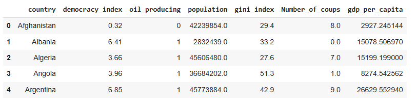
The NaN values in the ‘oil_producing’ and ‘Number_of_coups’ columns were filled with 0 to represent no oil or no coup. All other rows with NaN values were dropped.
Modeling
Random Forests
# select features and target from the dataset
# features
X = final.loc[:,['democracy_index', 'oil_producing',
'population','gini_index','Number_of_coups', 'gdp_per_capita']]
# target
y = final['coup']

# create the train and test split
X_train, X_test, y_train, y_test = train_test_split(X, y,
 test_size=0.3)

#import random forest model
from sklearn.ensemble import RandomForestClassifier

# create a Gaussian clasiffier
clf = RandomForestClassifier(n_estimators=100)

# Train the model using the training data
clf.fit(X_train, y_train)
y_predicted = clf.predict(X_test)

# model accuracy, how often is the classifier correct?
print('Accuracy: ', metrics.accuracy_score(y_test,
y_predicted))
Accuracy: 1.0
An accuracy of 1 means our model is perfect, but it could just be overfitting. So let’s try using cross validation.
# Using StratifiedKFold
from sklearn.model_selection import StratifiedKFold,
cross_val_score

# create train/test split - stratified
X_train, X_test, y_train, y_test = train_test_split(
    X, y, test_size=0.2, stratify=y, random_state=42
)

# set up StratifiedKFold CV for training set
skf = StratifiedKFold(n_splits=5, shuffle=True,
random_state=42)

# create model and run data
rf_model = RandomForestClassifier(random_state=42)
cv_scores = cross_val_score(rf_model, X_train,
y_train, cv=skf, scoring='accuracy')

print('CV accuracy per fold: ', cv_scores)
print('Mean CV accuracy: ', cv_scores.mean())

# fit model on full training set
rf_model.fit(X_train, y_train)

# Evaluate on holdout test set
test_accuracy = rf_model.score(X_test, y_test)
print('Holdout test accuracy:', test_accuracy)
CV accuracy per fold: [0.96 1. 1. 1. 1. ]
Mean CV accuracy: 0.992
Holdout test accuracy: 1.0
We get the same high accuracy even with cross-validation. Since the number of countries in the world is limited, we can increase the complexity if the data by increasing the columns to capture other dimesions of countries like the unemployment rate, the youth population, the average income, the economic comlplexity, the hapiness indes, the UN human development index, trade data, geographical data, poverty data etc.
Feature Importance
# feature importance on the basic random forest model
feature_imp = pd.Series(clf.feature_importances_,
index=X.columns).sort_values(ascending=False)
sns.barplot(x=feature_imp, y=feature_imp.index)
# Add labels to your graph
plt.xlabel('Feature Importance Score')
plt.ylabel('Features')
plt.title("Visualizing Important Features")
plt.legend()
plt.show()
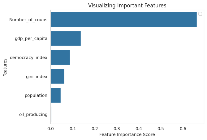
- From the bar chart above, the most important predictor for a coup is a history of previous coups. Remember at the beginning of this post when I said that the foiled Kenya Air Force coup of August 1982 would be important? This is it. The fact that the coup was unsuccessful meant that the chance of illegal and probably violent regime change was greatly reduced.
- The GDP per capita is the next most important factor, and it makes sense; the poorer a country is, the more likely that they are dissatisfied enough with the current regime to attempt a violent takeover.* Next is the democracy levels, which look obvious but are of lower importance. You would think that it would be a much more important factor, but just look at communist China, 2.11 on the democracy index, but never had a coup, and they are definitely getting richer (GPD per capita of $18820.51 in 2023).
- The wealth gap, as measured by the Gini index, is also surprisingly not that big a factor.
- The presence of natural resources is the lowest predictor, which seems to go against the literature; it seems you can’t always trust the machines.
Let us see what the cross-validated model has to say about feature importance.
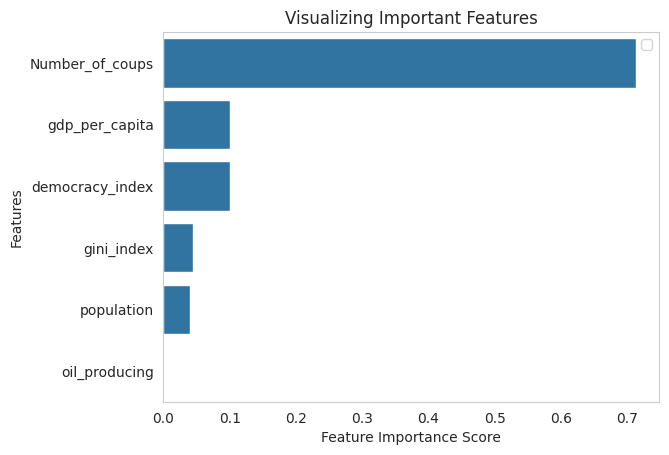
- Here we see a similar order, the top three most important factors are a history of coups, the country’s economic conditions and the democracy level. The presence of natural resources also features last here.
To predict whether a country may experience a coup, we need to pass its democracy index, whether it is oil-producing (1) or not (0), population, Gini index, number of coups, and GDP per capita in that order, to this prediction function.
# example prediction
clf.predict([[0.1, 1, 4569875, 64.5, 1, 956.32]])
array([1])
This predicts a coup in this fictitious country. Not surprising considering its abysmal democracy index, history of a coup and the low GDP per capita.
I will try this data on a linear regressor and a neural net to see how it plays out.